Global Irrigation Map, our capstone machine learning project
For our capstone project at UC Berkeley, we worked with the Department of Environmental Studies. We developed a machine learning model that we continued to improve even after the course term, and I’m happy to report that it is now under discussion to be a published paper – a first for the program itself, according to our lecturer.
Update Aug/5/2020: New blog post: a behind the scenes look on how we built the model.
About the project
In our project, we wanted to answer two key questions:
- How much of the world’s land is used as irrigated croplands?
- How has this changed over time? Are we having more or less land for irrigation?
This is an important question, because agriculture uses 70% of freshwater1. Any efficiencies we can bring in irrigation will directly improve how much water we will have for drinking and other domestic use.
A second reason is food security: between 2005 and 2050, studies estimate that food production needs to double to serve our growing population.2 That means more water: we need about 1 to 3 tons of water to grow a kilogram of cereal, and five times more water for a kilogram of beef.3
Therefore, we need to understand and improve how we use water for irrigation. Our project provides information about irrigation extent as well as trends, using satellite, climate and soil data, and machine learning models.
Results
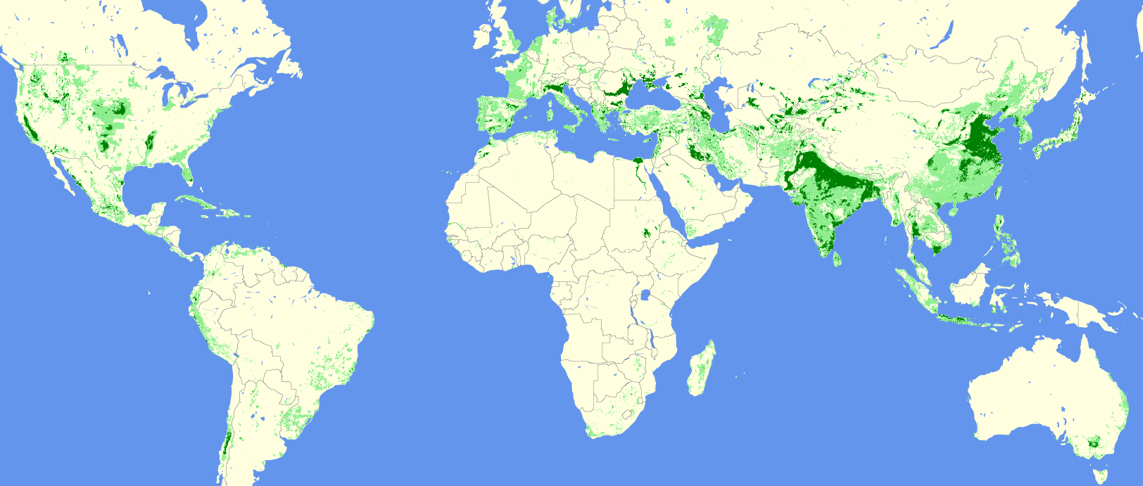
Our model predicted irrigation extent for the years 2000 through 2015, at a resolution of 9.3 km.
As of 2005, according to our model, 11% of the world’s land is irrigated croplands. Of this, 80% is in low-to-medium irrigation (<= 2000 hectares per 86 sq. km square of land), and the rest is high irrigation (>2000 hectares per 9.3km square of land).
Interactive irrigation extent map (2005):
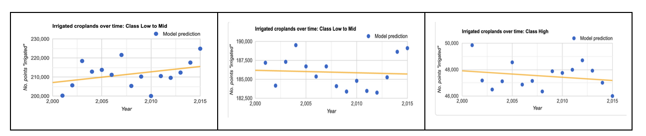
Between 2000 and 2015, irrigation decreased by 2% in the high irrigation category, but it increased by 4% in the lower end of irrigation.
Interactive irrigation change map, between 2000 and 2014:
Our model accuracy is 94%. Its kappa is 0.73. Our kappa value means that we are better than a model predicting based on irrigation frequency only, 73% of the time.
Interactive model assessment map (2005):
Methodology
I’ll now briefly describe technical details about the model and how we developed it.
Labels
We used Siebert’s Historical Irrigation Dataset (HID) 4 as labels for our models. This dataset contains irrigation data at 5 year intervals, as maximum area equipped for irrigation (in hectares) within each 9.3 by 9.3 km parcel of land globally.
Irrigation label distribution is highly concentrated at the lower end and falls off rapidly. This means most of our data is concentrated at the lower end. Also, irrigation is a small fraction of world’s land area so we have class imbalance.
Our final model combines two 2 different models: a time-stationary model and a time-series model.
Time-Stationary Model
The time-stationary model is a random-forest model that runs over all of the world’s continents except Antarctica. This can capture irrigation in the middle of Sahara desert, for example. We developed this as a large-scale machine learning model that runs on Google Earth Engine in a distributed fashion. We took a random sample of 20,000 points worldwide and used this sample for model development in R. We trained on 90% of this data, with 5-fold cross validation. We also used R to select features and classification algorithm, and tune its hyperparameters. We then ported the final model to GEE to run on the actual data. Its accuracy is 89% and kappa 0.56.
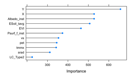
Our GEE model uses 9 features that vary in time, and 2 that capture time-invariant features: maximum temperature, evapotranspiration, downward surface shortwave radiation, wind-speed (all annual averages, TERRACLIMATE dataset); Albedo, direct evaporation from bare soil, atmospheric pressure, (all annual averages, GLDAS dataset); land-cover class, maximum EVI (MODIS datasets); latitude and longitude. Where the features differed in resolution, we reprojected to our label resolution of 9.3 km.
Time-Series Model
Our second model is a time-series model that pools labels from 1985 to 2000 inclusive. This model runs only on some parts of the world, namely areas already known to be croplands. We used GFSAD crop dominance data from 2010 to identify croplands. Applying this “cropland mask” reduced the data we process by 10X, and also allowed us to include more features in our label.
The time-series model uses a stacking approach. It initially runs an extra-trees classifier to check whether land is irrigated or not, at a threshold of 100 hectares. It then runs a second extra-trees classifier to differentiate within the first model’s predictions: none, low-to-medium (100 to 2000 ha), and high irrigation (> 2000 ha). To counter data imbalance, we under-sampled the non-irrigated class.
For features, we used NDVI (biannual mean, variance and maximum, AVHRR dataset); maximum temperature, minimum temperature, vapor pressure, downward surface shortwave radiation, wind-speed, actual evapotranspiration, climate water deficit, soil moisture (min, mean, max, variance, TERRACLIMATE dataset).
We developed the time-series model in Python with scikit-learn library, and ran it on a high-end virtual machine on Amazon cloud. Its accuracy is 89% and kappa 0.76.
We took a simple approach to combine the two models: for croplands, we use the time-series model. Everywhere else, we use the GEE model.
Validation
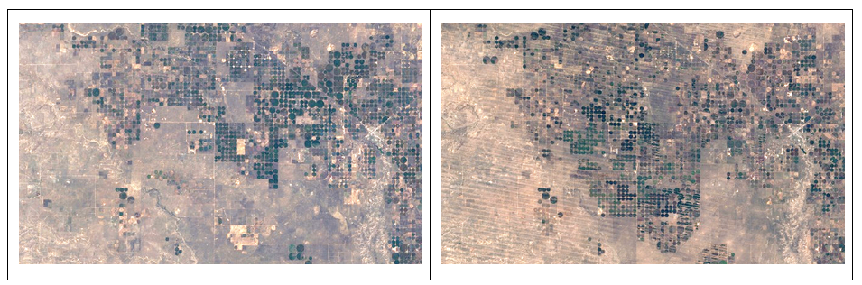
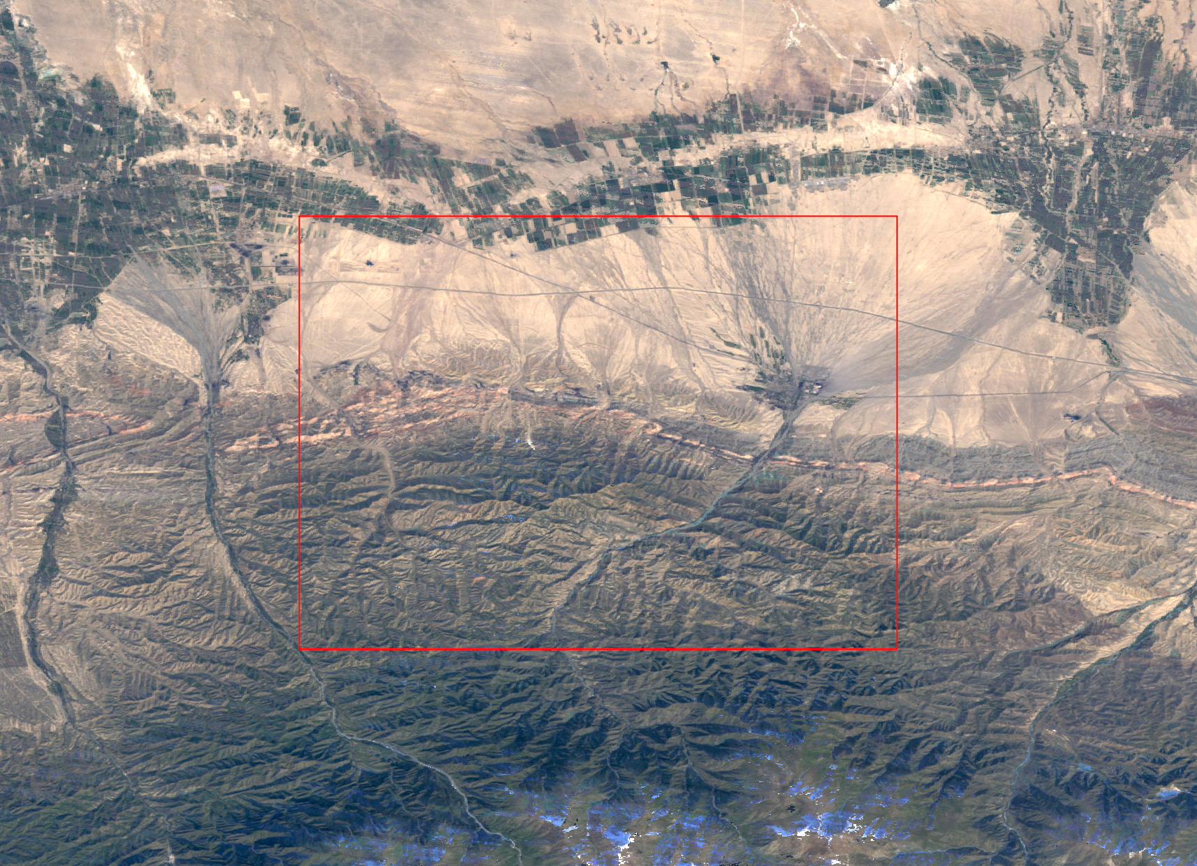
After running our model, we validated the false positives and false negatives produced by the model, by taking a random sample of 100 points in each class. We downloaded LANDSAT 7 TOA imagery for these points, for a radius of 9.3 km and a buffer of further 9.3 km. We then inspected each picture to validate the model classification.
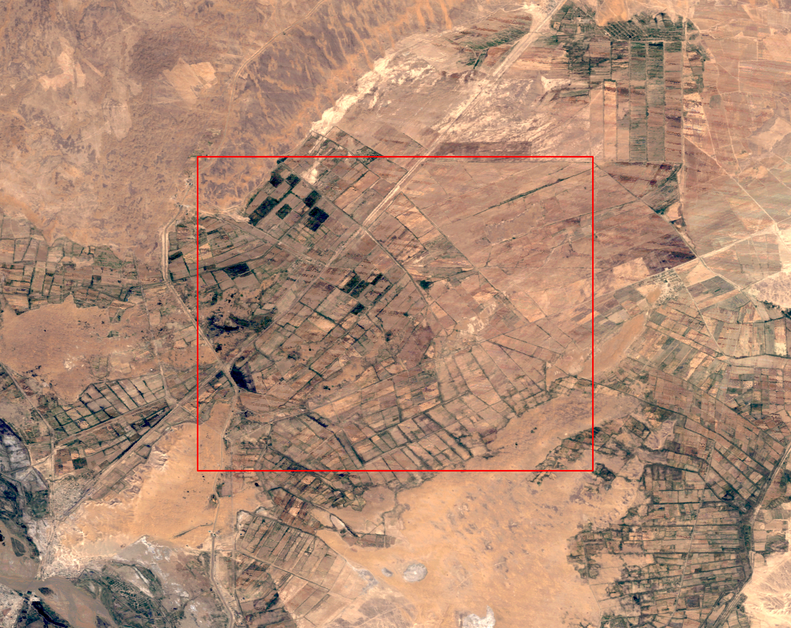
For points that are false positives, we found that 41 out of 100 points were croplands (27) or a mosaic of croplands and non-croplands such as hills, water bodies or forests (14). This means that the model was correct in its classification for these points. The remaining 59 points were non-croplands.
For points that are false negatives, we found that 47 out of 100 points were indeed non-croplands. This means the model was correct in its classification for these points. 33 points were a mosaic, and 20 points were croplands.
These numbers bring uncertainty to the model assessment metrics we state earlier based solely on the training labels.
Challenges
A key challenge in the project comes from the global scale. Because area grows quadratically (doubling the side quadruples the area), reducing spatial resolution becomes an engineering challenge more than a machine learning challenge. We chose to remain at 9.3km resolution in order to explore machine learning aspects of the project.
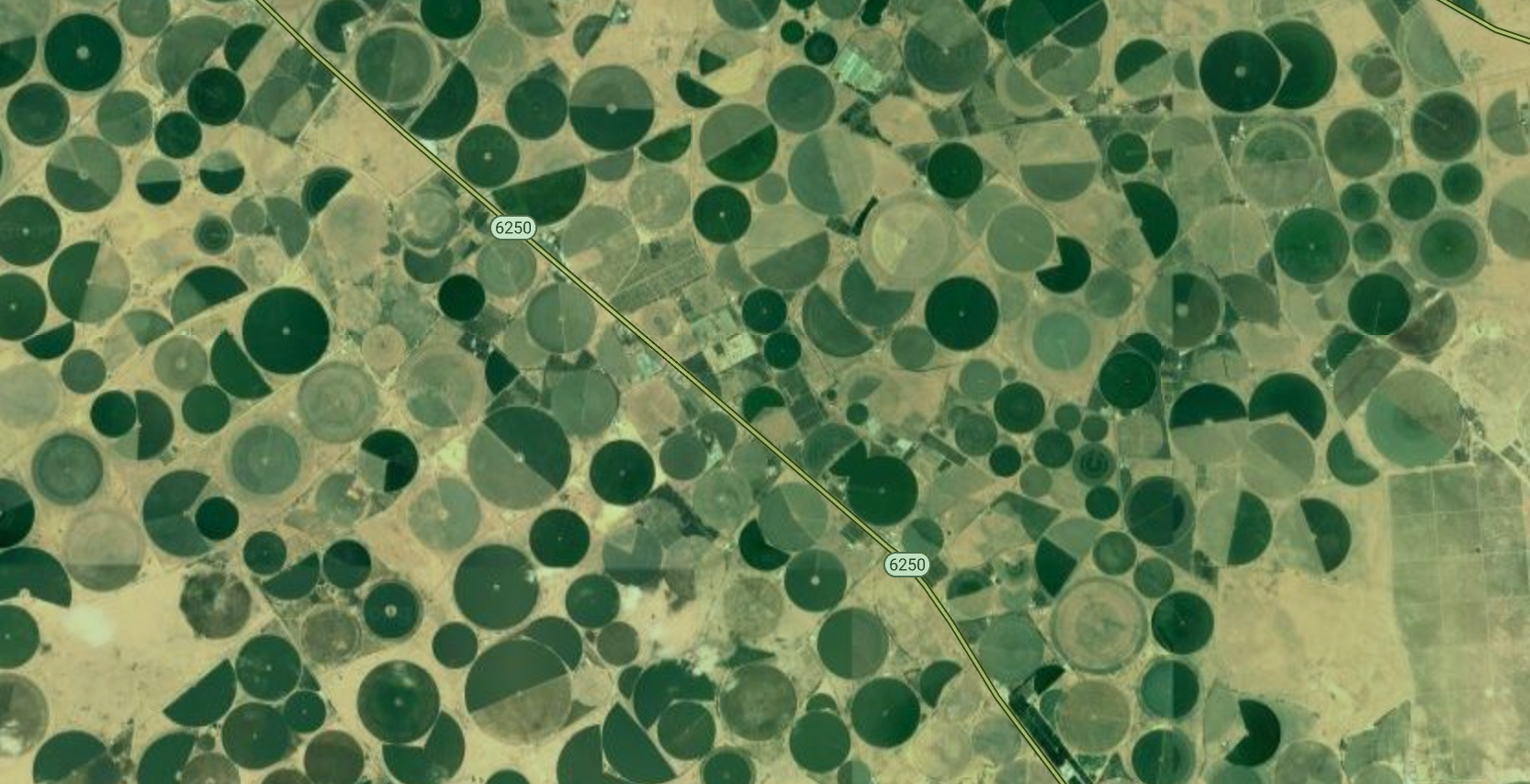
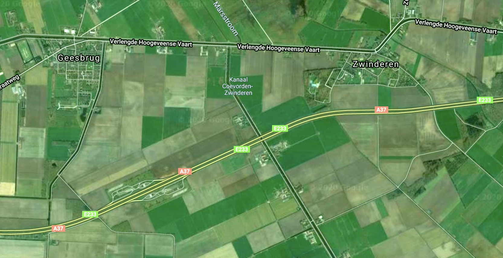
However, 9.3 by 9.3km is a large land area, and the terrain often does not let this whole area be croplands: there could be hills, ravines, rivers or lakes. In densely populated areas like India and China, holdings are small, unlike America. Such “mosaics” confuse the model and make it harder to distinguish between low and medium irrigation. This is one reason why we opted for a combined low-to-medium irrigation.
A second challenge is the inherent skew in data, which follows a power-law distribution: there are a few highly irrigated regions around major Himalayan rivers, Nile and the Mississippi, but the vast majority of irrigation is a small fraction. This also confuses the model.
An enhancement to the model would be to run it at finer resolution, say 500m or 1km, which could remove a lot of the mosaic-related problems. At this resolution, one could use a deep learning approach using satellite photography.
People and Credits
The problem was presented to us by our lecturer, Alberto Todeschini5. The researchers from environmental studies department were Prof. Paolo D’Odorico6 and Lorenzo Rosa7. Eleanor Proust8 developed the time-series model. I developed the time-stationary model.
Source code
Source code for the time-stationary GEE model is available at my Github repository9. I will make the time-series model also available there soon.
We presented an older version of our machine learning model for our capstone project coursework, which we have made available as a website.10
–
References
1 Source: FAO report, 2017
2 Tilman et al., 2011
3 Source: FAO report, 2017
4 Siebert et al., 2015
5 Alberto Todeschini
6 Paolo D’Odorico
7 Lorenzo Rosa
8 Eleanor Proust
9 Source code repository
10 Globalirrigationmap.org